Use case
Real-time High Dynamic Range Upconversion of Video
The following video demonstrates a real-time standard dynamic range (SDR) to high dynamic range (HDR) upconversion algorithm that was developed entirely in Quasar. The purpose of this algorithm is to display movies stored in SDR format on a HDR television. A user interface, also developed in Quasar, gives the user a few slides to choose how the conversion is done (e.g., which specular highlights are being boosted and to what extent).
"Raw upscaling" indicates direct scaling of the SDR to the HDR range, without additional processing of the video content. "Proposed method" refers to the SDR to HDR conversion algorithm.
(note: this video is played at a higher speed for viewing purposes)
Autonomous vehicles making use of Quasar
Simultaneous localization and mapping (SLAM)
Martin Dimitrievski and his colleagues propose a novel real-time method for SLAM in autonomous vehicles. The environment is mapped using a probabilistic occupancy map model and EGO motion is estimated within the same environment by using a feedback loop. Input data is provided via a rotating laser scanner as 3D measurements of the current environment which are projected on the ground plane. The local ground plane is estimated in real-time from the actual point cloud data using a robust plane fitting scheme. Then the computed occupancy map is registered against the previous map in order to estimate the translation and rotation of the vehicle. Experimental results demonstrate that the method produces high quality occupancy maps and the measured translation and rotation errors of the trajectories are lower compared to other 6 degrees of freedom methods. The entire SLAM system runs on a mid-range GPU and keeps up with the data from the sensor which enables more computational power for the other tasks of the autonomous vehicle.
“Many of the Autonomous Vehicles sub-systems are massively parallel and this is where Quasar can speed things up. From pre-processing of LIDAR point cloud data to odometry, object detection, tracking and route planning, Quasar made all of these components possible to run on a mid-range GPU in real-time. When you are done prototyping, you can consult the profiler to easily spot any areas for improved execution of the code.” – ir. Martin Dimitrievski
Example: SLAM for autonomous vehicles
Reference
“Robust matching of occupancy maps for odometry in autonomous vehicles“; Martin Dimitrievski , David Van Hamme , Peter Veelaert, Wilfried Philips in
proceedings of Joint Conference on Computer Vision, Imaging and Computer Graphics Theory and Applications 2016 (VISIGRAPP).
Acknowledgements
The work was financially supported the Flanders Make ICON project 140647 “Environmental Modelling for automated Driving and Active Safety (EMDAS)”.
MRI reconstruction speedups up to x20 using GPUs
Magnetic Resonance Imaging (MRI)
MRI is a very powerful and safe medical diagnostic tool, but it is prohibitively expensive to use frequently. Hence, a technique that speeds up MRI acquisition would not only be helpful for patients, as it requires them to lie still for shorter periods of time, but it would also be of great benefit for doctors, as it leads to a higher patient throughput and a reduced susceptibility of the images to motion artifacts. Using Quasar, Jan Aelterman and his colleagues developed a reconstruction algorithm that handles acquisition speedup correctly.
Speeding up MRI is done by reducing the amount of acquired data. However, signal processing theory states it is impossible to do this beyond the Nyquist limit, without losing information. However, it is possible to only lose superfluous image information, this is called compressive sensing (CS). The danger is that that a naive reconstruction technique inadvertently corrupts an image while filling in lost information.
Proposed Technique
An MRI image is constructed from so called Fourier, or k-space coefficients. Due to acceleration techniques, the number of Fourier coefficients is less than the number of image pixels, resulting in an infinite number of possible images that would correspond with the acquired Fourier coefficients (an infinite number of ways to fill in the missing, superfluous information). Therefore, we impose an additional constraint: the reconstructed image is the one with the lowest number of shearlet coefficients possible. The shearlet transform can represent natural images with few coefficients, but not noise and corruptions. It is optimal in this respect. Hence, its use will force a noise – and corruption – free reconstruction. The optimization of the proposed problem requires iteratively applying the Non-uniform fast Fourier transform (NUFFT), which after profiling turns out to be a major bottleneck. By accelerating the NUFFT using the GPU we are able to gain significant speedups.
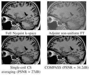
COMPASS reconstruction experiment using 4 acquisition coils and 10% of the Nyquist sampling rate on a k-space spiral.
Implementation was done using the new programming language Quasar, which allows for fast and hardware agnostic development, while still using the computation power of the GPU. Without requiring long development cycles, we were able to achieve speed-ups up to a factor 20 on an NVIDIA Geforce GTX 770. The speed-up achieved by the GPU acceleration opens the path for new and innovative research for MRI reconstruction: e.g. auto calibration, 3D reconstruction, advanced regularization parameters, etc.
“It took experts using CUDA/C++ three months to implement our MRI reconstruction algorithm; a developer using Quasar for the very first time achieved the same numerical results at the same computational performance in less than a single development week.” – Dr. ir. Jan Aelterman
Example
Reference
“COMPASS: a joint framework for parallel imaging and compressive sensing in MRI“; Jan Aelterman, Quang Luong, Bart Goossens, Aleksandra Pizurica, Wilfried Philips; in proceedings of IEEE International Conference on Image Processing ICIP(2010).
Focal Black & White effect
Focal Black & White Effect
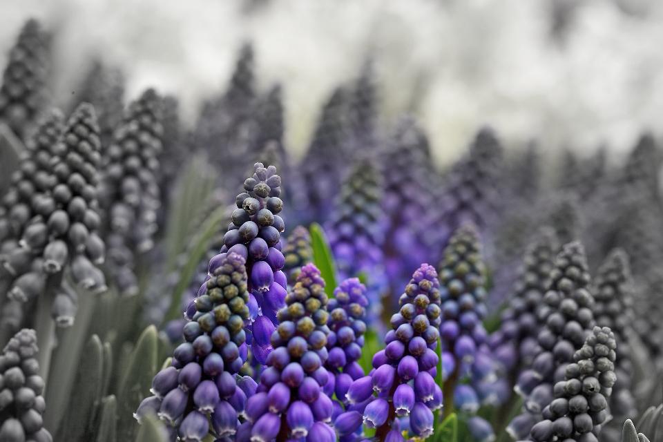
A well known Google Picasa effect is the Focal Black & White Effect. This effect preserves the color within a focal region and converts pixels outside this region to grayscale.
The algorithm is surprisingly simple: it consists of calculating a weighting factor (that depends on the focal radius), converting the pixel RGB values at each position to grayscale, and calculating a weighted average of this value with the original RGB value. Let us see how this can be achieved in Quasar:
function [] = __kernel__ focus_bw(x, y, focus_spot, falloff, radius, pos)

    % Calculation of the weight
    p = (pos - focus_spot) / max(size(x,0..1))
    weight = exp(-1.0 / (0.05 + radius * (2 * dotprod(p,p)) ^ falloff))

    % Conversion to grayscale & averaging
    rgbval = x[pos[0],pos[1],0..2]
    grayval = dotprod(rgbval,[0.3,0.59,0.11])*[1,1,1]
    y[pos[0],pos[1],0..2] = lerp(grayval, rgbval, weight)

end
Code explanation
First, the kernel function focus_bw is defined. __kernel__ is a special function qualifier that identifies a kernel function (similar to OpenCL’s __kernel or kernel qualifier). Kernel functions are natively compiled to any target architecture that you have in mind. This can be multi-core CPU x86/64 ELF, even ARM v9 with Neon instructions; up to NVidia PTX code. Next, a parameter list follows, the type of the parameters is (in this case) not specified.
Note the special parameter pos. In Quasar, pos is a parameter name that is reserved for kernel functions to obtain the current position in the image.
The kernel function contains two major blocks:
- In the weight calculation step, first the relative position compared to the focus spot coordinates is computed. This relative position is normalized by dividing by the maximum size in the first two dimensions (note that Quasar uses base-0), so this is the maximum of the width and the height of the image. Next, the weight is obtained as being inversely proportional to distance to the the focal spot. A special built-in function
dotprod, that can also be found in high-level shader languages (HLSL/GLSL) and that calculates the dot product between two vectors, is used for this purpose. - For extracting the RGB value at the position
pos, we use a matrix slice indexer:0..2constructs a vector of length 3 (actually[0,1,2]), which vector is used for indexing. In fact:x[pos[0],pos[1],0..2] = [x[pos[0],pos[1],0],x[pos[0],pos[1],1],x[pos[0],pos[1],2]]which form do you prefer, the left-handed side, or the right-handed side? You can choose. Note that it is not possible to write:
x[pos[0..1],0..2], because this expression would construct a matrix of size2 x 3. - The gray value is calculated by performing the dot product of
[0.3,0.59,0.11]with the original RGB value. Finally, the gray value is mixed with the original RGB value using thelerp“linear interpolation” function. In fact,lerpis nothing more than the function:lerp = (x,y,a) -> (1-a) * x + a * xThe resulting RGB value is written to the output image
y. That’s it!
Finally, we still need to call the kernel function. For this, we use the parallel_do construct:
img_in = imread("quasar.jpg")
img_out = zeros(size(img_in))

parallel_do(size(img_out,0..1),img_in,img_out,[256,128],0.5,10,focus_bw)
imshow(img_out)
First, an input image img_in is loaded using the function imread “image read”. Then, an output image is allocated with the same size as the input image.
The parallel_do function is called, with some parameters. The first parameter specifies the dimensions of the “work items” that can run in parallel. Here, each pixel of the image can be processed in parallel, hence the dimensions are the size (i.e., height + width) of the output image. The following parameters are argument values that are passed to the kernel function and that are declared in the kernel function definition. Finally, the kernel function to be called is passed.
Note that in contrast to scripting languages that are dynamically typed, the Quasar language is (mostly) statically typed and the Quasar compiler performs type inference in order to derive the data types of all the parameters. This is done based on the surrounding context. Here, Quasar will find out that img_in is a cubedata type (a 3D array) and it will derive all other missing data types based on that. Consequently, efficient parallel code can be generated in a manner that is independent of the underlying platform.
Now: the complete code again:
function [] = __kernel__ focus_bw(x, y, focus_spot, falloff, radius, pos)
    p = (pos - focus_spot) / max(size(x,0..1))
    weight = exp(-1.0 / (0.05 + radius * (2 * dotprod(p,p)) ^ falloff))
    rgbval = x[pos[0],pos[1],0..2]
    grayval = dotprod(rgbval,[0.3,0.59,0.11])*[1,1,1]
    y[pos[0],pos[1],0..2] = lerp(grayval, rgbval, weight)
end

img_in = imread("flowers.jpg")
img_out = zeros(size(img_in))

parallel_do(size(img_out,0..1),img_in,img_out,[256,128],0.5,10,focus_bw)
imshow(img_out)
Example
With eleven lines of code, you have a beautifully shining Focal Black & White effect:
Quasar facilitates research on video analysis.
Optical Flow
Simon Donné and his colleagues achieved significant speed-ups for Optical Flow, a widely used video analysis method, thanks to the use of GPUs and Quasar. Tracking an object through time is often still a hard task for a computer. One option is to use optical flow, which finds correspondences between two image frames: which pixel moves where? In general, these techniques compare local neighbourhoods and exploit global information to estimate these correspondences. The authors presented their new approach at the conference for Advanced Concepts for Intelligent Vision Systems (ACIVS) in Catania, Italy.
“Thanks to the Quasar platform we have both a CPU and GPU implementation of the approach. Therefore we achieve a speed-up factor of more than 40 compared to the existing pixel-based method” – ir. Simon Donné
Example
Reference
“Fast and Robust Variational Optical Flow for High-Resolution Images using SLIC Superpixels“; Simon Donné, Jan Aelterman, Bart Goossens, Wilfried Philips in Lecture Notes in Computer Science, Advanced Concepts for Intelligent Vision Systems, 2015

3D Real-time video processing demo
In this post, we demonstrate some of the real-time video processing and visualization capabilities of Quasar. Initially, a monochromatic image and corresponding depth image were captured using a video camera. Because the depth image is originally quite noisy, some additional processing is required. To visualize the results in 3D, we define a fine rectangular mesh in which the z-coordinate of each vertex is set to the depth value at position (x,y). All processing is automatically performed on the GPU and the result is visualized through the integrated OpenGL support in Quasar.
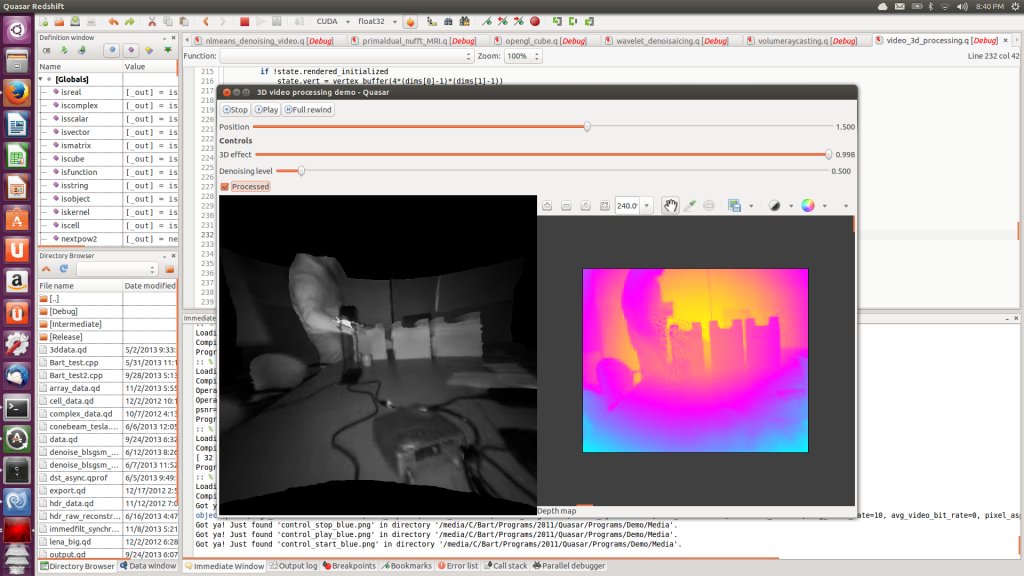
Ubuntu screenshot of the depth image denoising application
The demonstration video first shows the different parts of this video processing algorithm: first the non-local means denoising algorithm used for processing depth images, second the rendering functionality (through OpenGL vertex buffers) and finally, the user interface code (with sliders, labels and displays).
When the program runs, first a flat 2D image is shown on the left, together with the depth image on the right. By adjusting the “3D” slider, the flat image is extruded to a 3D surface.
It can be seen that there are some problems in the resulting 3D mesh, especially in the vicinity of right hand of the test subject. These problems are caused by reflective properties of the desk lamp standing in between the subject and the camera. By increasing the denoising level of the algorithm, this problem can easily be solved. Although the 3D surface has a much smoother appeareance, the depth image on the right reveals that the depth image is actually over-smoothed. The right balance between smoothing and local surface artifacts can be found by setting the denoising level somewhere “in the middle”.