How to’s
The Three Function Types of Quasar from a Technical Perspective
To give programmers ultimate control on the acceleration of functions on compute devices (GPU, multi-core CPU), Quasar has three distinct function types:
- Host Functions: host functions are the default functions in Quasar. Depending on the compilation target, they are either interpreted or compiled to binary CPU code. Host functions run on the CPU and form a glue for the code that runs on other devices. When host functions contain for-loops, these loops are (when possible) automatically parallelized by the Quasar compiler. The parallelized version then runs on multi-core CPU or GPU; what happens in the background is that a kernel function is generated. Within the Quasar Redshift IDE, host functions are interpreted, which also allows stepping through the code and putting breakpoints.
- Kernel Functions: given certain data dimensions, kernel functions specify what needs to be done to each element of the data. The task can be either a parallel task or a serial task. Correspondingly, kernel functions are launched either using the
parallel_dofunction or using theserial_dofunction:function [] = __kernel__ filter(image, pos) ... endfunction parallel_do(size(image),image,filter)In the above example, the kernel function
filteris applied in parallel to each pixel component of the imageimage. The first parameter ofparallel_do/serial_dois always the data dimension (i.e., the size of the data). The last parameter is the kernel function to be called, and in the middle are the parameters to be passed to the kernel function.posis a special kernel function parameter that indicates the position within the data (several other parameters exist, such asblkpos,blkdimetc., see the documentation for a detailed list).Kernel functions can call other kernel functions, but only through
serial_doand/orparallel_do. The regular function calling syntax (direct call, i.e, withoutserial_do/parallel_do) on kernel functions is not permitted. This is because kernel functions have other infrastructure (e.g., shared memory, device-specific parameters) which would cause conflicts when kernel functions would call each other. - Device functions: in contrast to host functions, device functions (indicated with
__device__) are intended to be natively compiled using the back-end compiler. They can be seen as auxiliary functions that can be called from either kernel functions, device functions or even host functions (note that a kernel function cannot call a host function). The compiler back-end may generate C++, CUDA or OpenCL code that is then further compiled to binary code to be executed on CPU and/or GPU. Currently, apart from the CPU there are no accelerators that can run a device function directly when called from a host function. This means, for a GPU, the only way to call a device function is through a kernel function.function y = __device__ norm(vector : vec) y = sqrt(sum(vector.^2)) endfunction
Functions in Quasar are first-class variables. Correspondingly, they have a data type. Below are some example variable declarations:
host : [(cube, cube) -> scalar]
filter : [__kernel__ (cube) -> ()]
norm : [__device__ (vec) -> scalar]
This allows passing functions to other functions, where the compiler can statically check the types. Additionally, to prevent functions from being accessed unintendedly, functions can be nested. For example, a gamma correction operation can be implemented using a host function containing a kernel function.
    function y : mat = gamma_correction(x : mat, gamma_fn : [__device__ scalar->scalar])
        function [] = __kernel__ my_kernel(gamma_fn : [__device__ scalar->scalar], x : cube, y : cube, pos : ivec2)
           y[pos] = gamma_fn(x[pos])
        endfunction
        y = uninit(size(x)) % Allocation of uninitialized memory
        parallel_do(size(x), gamma_fn, x, y, my_kernel)
    endfunction
Because functions support closures (i.e., they capture the variable values of the surround contexts at the moment the function is defined), the above code can be simplified to:
    function y : mat = gamma_correction(x : mat, gamma_fn : [__device__ scalar->scalar])
        function [] = __kernel__ my_kernel(pos : ivec2)
           y[pos] = gamma_fn(x[pos])
        endfunction
        y = uninit(size(x))
        parallel_do(size(x), my_kernel)
    endfunction
Or even in shorter form, using lambda expression syntax:
function y : mat = gamma_correction(x : mat, gamma_fn : [__device__ scalar->scalar])
    y = uninit(size(x))
    parallel_do(size(x), __kernel__ (pos) -> y[pos] = gamma(x[pos]))
end
In many cases, the type of the variables can safely be omitted (e.g., pos in the above example) because the compiler can deduce it from the context.
Now, experienced GPU programmers may wonder about the performance cost of a function pointer call from a kernel function. The good news is that the function pointer call is avoided, by automatic function specialization (a bit similar to template instantiation in C++). With this mechanism, device functions passed via the function parameters or closure can automatically be inlined in a kernel function.
function y = gamma_correction(x, gamma_fn)
    y = uninit(size(x))
    parallel_do(size(x), __kernel__ (pos) -> y[pos] = gamma(x[pos]))
end
gamma = __device__ (x) -> 255*(x/255)^2.4
im_out = gamma_correction(im_in, gamma)
This will cause the following kernel function to be generated, behind the hood:
function [] = __kernel__ opt__gamma_correction(pos:int,y:vec,x:vec)
      % Inlining of function 'gamma' with parameters 'x'=x[pos]
      y[pos]=(255*((x[pos]/255)^2.4))
endfunction
Another optimization was performed in the background: kernel flattening. Because each element of the data is accessed separately, the data is processed as a vector (using raster scanning) rather than as a matrix (or cube) representation. This entirely eliminates costly index calculations.
Summarizing, three function types offer the flexibility of controlling on which target devices (CPU or GPU) certain code fragments might run, while offering a unified programming interface: the code written for GPU can be executed on CPU as well, thereby triggering other target-specific optimizations.
Focal Black & White effect
Focal Black & White Effect
A well known Google Picasa effect is the Focal Black & White Effect. This effect preserves the color within a focal region and converts pixels outside this region to grayscale.
The algorithm is surprisingly simple: it consists of calculating a weighting factor (that depends on the focal radius), converting the pixel RGB values at each position to grayscale, and calculating a weighted average of this value with the original RGB value. Let us see how this can be achieved in Quasar:
function [] = __kernel__ focus_bw(x, y, focus_spot, falloff, radius, pos)

    % Calculation of the weight
    p = (pos - focus_spot) / max(size(x,0..1))
    weight = exp(-1.0 / (0.05 + radius * (2 * dotprod(p,p)) ^ falloff))

    % Conversion to grayscale & averaging
    rgbval = x[pos[0],pos[1],0..2]
    grayval = dotprod(rgbval,[0.3,0.59,0.11])*[1,1,1]
    y[pos[0],pos[1],0..2] = lerp(grayval, rgbval, weight)

end
Code explanation
First, the kernel function focus_bw is defined. __kernel__ is a special function qualifier that identifies a kernel function (similar to OpenCL’s __kernel or kernel qualifier). Kernel functions are natively compiled to any target architecture that you have in mind. This can be multi-core CPU x86/64 ELF, even ARM v9 with Neon instructions; up to NVidia PTX code. Next, a parameter list follows, the type of the parameters is (in this case) not specified.
Note the special parameter pos. In Quasar, pos is a parameter name that is reserved for kernel functions to obtain the current position in the image.
The kernel function contains two major blocks:
- In the weight calculation step, first the relative position compared to the focus spot coordinates is computed. This relative position is normalized by dividing by the maximum size in the first two dimensions (note that Quasar uses base-0), so this is the maximum of the width and the height of the image. Next, the weight is obtained as being inversely proportional to distance to the the focal spot. A special built-in function
dotprod, that can also be found in high-level shader languages (HLSL/GLSL) and that calculates the dot product between two vectors, is used for this purpose. - For extracting the RGB value at the position
pos, we use a matrix slice indexer:0..2constructs a vector of length 3 (actually[0,1,2]), which vector is used for indexing. In fact:x[pos[0],pos[1],0..2] = [x[pos[0],pos[1],0],x[pos[0],pos[1],1],x[pos[0],pos[1],2]]which form do you prefer, the left-handed side, or the right-handed side? You can choose. Note that it is not possible to write:
x[pos[0..1],0..2], because this expression would construct a matrix of size2 x 3. - The gray value is calculated by performing the dot product of
[0.3,0.59,0.11]with the original RGB value. Finally, the gray value is mixed with the original RGB value using thelerp“linear interpolation” function. In fact,lerpis nothing more than the function:lerp = (x,y,a) -> (1-a) * x + a * xThe resulting RGB value is written to the output image
y. That’s it!
Finally, we still need to call the kernel function. For this, we use the parallel_do construct:
img_in = imread("quasar.jpg")
img_out = zeros(size(img_in))

parallel_do(size(img_out,0..1),img_in,img_out,[256,128],0.5,10,focus_bw)
imshow(img_out)
First, an input image img_in is loaded using the function imread “image read”. Then, an output image is allocated with the same size as the input image.
The parallel_do function is called, with some parameters. The first parameter specifies the dimensions of the “work items” that can run in parallel. Here, each pixel of the image can be processed in parallel, hence the dimensions are the size (i.e., height + width) of the output image. The following parameters are argument values that are passed to the kernel function and that are declared in the kernel function definition. Finally, the kernel function to be called is passed.
Note that in contrast to scripting languages that are dynamically typed, the Quasar language is (mostly) statically typed and the Quasar compiler performs type inference in order to derive the data types of all the parameters. This is done based on the surrounding context. Here, Quasar will find out that img_in is a cubedata type (a 3D array) and it will derive all other missing data types based on that. Consequently, efficient parallel code can be generated in a manner that is independent of the underlying platform.
Now: the complete code again:
function [] = __kernel__ focus_bw(x, y, focus_spot, falloff, radius, pos)
p = (pos - focus_spot) / max(size(x,0..1))
weight = exp(-1.0 / (0.05 + radius * (2 * dotprod(p,p)) ^ falloff))
rgbval = x[pos[0],pos[1],0..2]
grayval = dotprod(rgbval,[0.3,0.59,0.11])*[1,1,1]
y[pos[0],pos[1],0..2] = lerp(grayval, rgbval, weight)
end
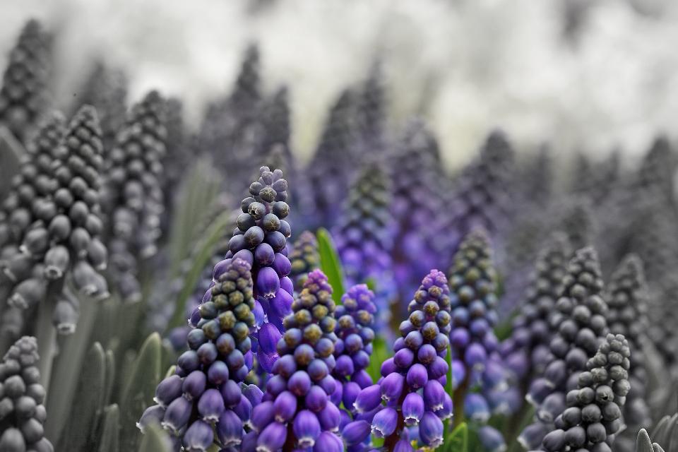
img_in = imread("flowers.jpg")
img_out = zeros(size(img_in))
parallel_do(size(img_out,0..1),img_in,img_out,[256,128],0.5,10,focus_bw)
imshow(img_out)
Example
With eleven lines of code, you have a beautifully shining Focal Black & White effect:
Quasar for Matlab/Octave users
This section gives an overview of various functions and operators in Matlab and Quasar. Please feel free to extend this page if you find something that is missing.
Quick hints (see reference manual for a complete description):
- Matrices are passed by reference rather than by value. If necessary, use the
copy(.)function. - Indices start with 0 rather than with 1.
endvariable, like inA(end,end)is currently not supported.- All functions work transparently on the GPU (in MATLAB you need to use special datatypes
GPUsingle,GPUdouble, …)
Arithmetic operators
| MATLAB/Octave | Quasar | |
| Assignment | a=1; b=2; | a=1; b=2 |
| Multiple assignment | [a,b]=[1,2]; | [a,b]=[1,2] |
| Addition | a+b | a+b |
| Subtraction | a-b | a-b |
| Multiplication | a*b | a*b |
| Division | a/b | a/b |
| Power | a^b | a^b |
| Remainder | rem(a,b) | periodize(a,b) |
| Addition (atomic) | a+=1 | a+=1 |
| Pointwise multiplication | a.*b | a.*b |
| Pointwise division | a./b | a./b |
| Pointwise power | a.^b | a.^b |
Relational operators
| MATLAB/Octave | Quasar | |
| Equality | a==b | a==b |
| Less than | a < b | a < b |
| Greater than | a > b | a > b |
| Less than or equal | a <= b | a <= b |
| Greater than or equal | a >= b | a >= b |
| Inequal | a ~= b | a != b |
Logical operators
| MATLAB/Octave | Quasar | |
| Logical AND | a && b | a && b |
| Logical OR | a || b | a || b |
| Logical NOT | ~a | !a |
| Logical XOR | xor(a,b) | xor(a,b) |
| Bitwise AND | a & b | and(a,b) |
| Bitwise OR | a | b | or(a,b) |
| Bitwise NOT | ~a | not(a) |
| Bitwise XOR | xor(a,b) | xor(a,b) |
Square root, logarithm
| MATLAB/Octave | Quasar | |
| Square root | sqrt(a) | sqrt(a) |
| Logarithm, base e | log(a) | log(a) |
| Logarithm, base 2 | log2(a) | log2(a) |
| Logarithm, base 10 | log10(a) | log10(a) |
| Exponential function | exp(a) | exp(a) |
Rounding
| MATLAB/Octave | Quasar | |
| Round | round(a) | round(a) |
| Round up | ceil(a) | ceil(a) |
| Round down | floor(a) | floor(a) |
| Round towards zero | fix(a) | Not implemented yet |
| Fractional part | frac(a) | frac(a) |
Mathematical constants
| MATLAB/Octave | Quasar | |
| pi | pi | pi |
| e | exp(1) | exp(1) |
Missing values (IEEE-754 floating point status flags)
| MATLAB/Octave | Quasar | |
| Not a number | NaN | 0/0 |
| +Infinity | +inf | 1/0 |
| -Infinity | -inf | -1/0 |
| Is not a number | isnan(x) | isnan(x) |
| Is infinity | isinf(x) | isinf(x) |
| Is finite | isfinite(x) | isfinite(x) |
Complex numbers
| MATLAB/Octave | Quasar | |
| Imaginary unit | i | 1i or 1j |
| Complex number 3+4i | z=3+4i | z=3+4i or z=complex(3,4) |
| Modulus | abs(z) | abs(z) |
| Argument | arg(z) | angle(z) |
| Real part | real(z) | real(z) |
| Imaginary part | imag(z) | imag(z) |
| Complex conjugate | conj(z) | conj(z) |
Trigonometry
| MATLAB/Octave | Quasar | |
| Sine | sin(x) | sin(x) |
| Cosine | cos(x) | cos(x) |
| Tangent | tan(x) | tan(x) |
| Hyperbolic Sine | sinh(x) | sinh(x) |
| Hyperbolic Cosine | cosh(x) | cosh(x) |
| Hyperbolic Tangent | tanh(x) | tanh(x) |
| Arcus Sine | asin(x) | asin(x) |
| Arcus Cosine | acos(x) | acos(x) |
| Arcus Tangent | atan(x) | atan(x) |
| Arcus Hyperbolic Sine | asinh(x) | asinh(x) |
| Arcus Hyperbolic Cosine | acosh(x) | acosh(x) |
| Arcus Hyperbolic Tangent | atanh(x) | atanh(x) |
Random numbers
| MATLAB/Octave | Quasar | |
| Uniform distribution [0,1[ | rand(1,10) | rand(1,10) |
| Gaussian distribution | randn(1,10) | randn(1,10) |
| Complex Gaussian distribution | randn(1,10)+1i*randn(1,10) | complex(randn(1,10),randn(1,10)) |
Vectors
| MATLAB/Octave | Quasar | Comment | |
| Row vector | a=[1 2 3 4]; | a=[1,2,3,4] | |
| Column vector | a=[1; 2; 3; 4]; | a=transpose([1,2,3,4]) | |
| Sequence | 1:10 | 1..10 | |
| Sequence with steps | 1:2:10 | 1..2..10 | |
| Decreasing sequence | 10:-1:1 | 10..-1..1 | |
| Linearly spaced vectors | linspace(1,10,5) | linspace(1,10,5) | |
| Reverse | reverse(a) | reverse(a) | import “system.q” |
Concatenation
Quasar notes: please avoid because this programming approach is not very efficient. More efficient is to create the resulting matrix using zeros(x), then use slice accessors to fill in the different parts.
| MATLAB/Octave | Quasar | Comments | |
| Horizontal concatenation | [a b] | cat(a,b) | import “system.q” |
| Vertical concatenation | [a; b] | vertcat(a,b) | import “system.q” |
| Vertical concatenation with sequences | [0:5; 6:11] | vertcat(0..5,6..11) | import “system.q” |
| Repeating | repmat(a,[1 2]) | repmat(a,[1,2]) |
Matrices
| MATLAB/Octave | Quasar | Comment | |
| The first 10 element X+Y | a(1:10,1:10); | a[0..9,0..9] | |
| Skip the first elements X+Y | a(2:end,2:end); | a[1..size(a,0)-1,1..size(a,1)-1] | |
| The last elements | a(end,end) | a[size(a,0..1)-1] | |
| 10th row | a(10,:) | a[9,:] | |
| 10th column | a(:,10) | a[:,9] | |
| Diagonal elements | diag(a) | diag(a) | import “system.q” |
| Matrix with diagonal 1,2,…,10 | diag(1..10) | diag(0..9) | import “system.q” |
| Reshaping | reshape(a,[1 2 3]) | reshape(a,[1,2,3]) | |
| Transposing | transpose(a) | transpose(a) | |
| Hermitian Transpose | a’ | herm_transpose(a) | import “system.q” |
| Copying matrices | a=b | a=copy(b) | Matrices passed by reference for efficiency |
| Flip upsize-down | flipud(a) | flipud(a) | |
| Flip left-right | fliplr(a) | fliplr(a) |
Matrix dimensions
| MATLAB/Octave | Quasar | Comments | |
| Number of elements | numel(a) | numel(a) | |
| Number of dimensions | ndims(a) | ndims(a) | import “system.q” |
| Size | size(a) | size(a) | |
| Size along 2nd dimension | size(a,2) | size(a,1) | |
| Size along 2nd & 3rd dimension | [size(a,2),size(a,3)] | size(a,1..2) |
Array/matrix creation
| MATLAB/Octave | Quasar | Comment | |
| Identity matrix | eye(3) | eye(3) | |
| Zero matrix | zeros(2,3) | zeros(2,3) | |
| Ones matrix | ones(2,3) | ones(2,3) | |
| Uninitialized matrix | – | uninit(2,3) | |
| Complex identity matrix | complex(eye(3)) | complex(eye(3)) | |
| Complex zero matrix | complex(zeros(2,3)) | czeros(2,3) | |
| Complex ones matrix | complex(ones(2,3)) | complex(ones(2,3)) | |
| Complex Uninitialized matrix | – | cuninit(2,3) | |
| Vector | zeros(1,10) | zeros(10) or vec(10) | vec enables generic programming |
| Matrix | zeros(10,10) | zeros(10,10) or mat(10,10) | mat enables generic programming |
| Cube | zeros(10,10,10) | zeros(10,10,10) or cube(10,10,10) | cube enables generic programming |
Maximum and minimum
| MATLAB/Octave | Quasar | |
| Maximum of two values | max(a,b) | max(a,b) |
| Minimum of two values | min(a,b) | min(a,b) |
| Maximum of a matrix | max(max(a)) | max(a) |
| Minimum of a matrix along dimension X=1,2 | min(a,[],X) | min(a,X-1) |
| Maximum of a matrix along dimension X=1,2 | max(a,[],X) | max(a,X-1) |
Matrix assignment
| MATLAB/Octave | Quasar | Comments | |
| Assigning a constant to a matrix slice | a(:,1)=44; | a[:,0]=44 | |
| Assigning a vector to a matrix row slice | a(:,1)=0:99 | a[:,0]=0..99 | |
| Assigning a vector to a matrix column slice | a(1,:)=(0:99)’ | a[0,:]=transpose(0..99) | |
| Replace all positive elements by one | a(a>0)=1 | a[a>0]=1 | *New* |
Boundary handling, clipping (coordinate transforms)
| MATLAB/Octave | Quasar | Comments | |
| Periodic extension | rem(x,N) | periodize(x,N) | |
| Mirrored extension | – | mirror_ext(x,N) | |
| Clamping | – | clamp(x,N) | returns 0 when x=N, otherwise x. |
| Saturation between 0 and 1 | – | sat(x) | returns 0 when x=1, otherwise x. |
Fourier transform
| MATLAB/Octave | Quasar | Comments | |
| 1D FFT | fft(x) | fft1(x) | |
| 2D FFT | fft2(x) | fft2(x) | |
| 3D FFT | fftN(x) | fft3(x) | |
| 1D inverse FFT | ifft(x) | ifft1(x) | |
| 2D inverse FFT | ifft2(x) | ifft2(x) | |
| 3D inverse FFT | ifftN(x) | ifft3(x) | |
| 1D fftshift | fftshift(x) | fftshift1(x) | import “system.q” |
| 2D fftshift | fftshift(x) | fftshift2(x) | import “system.q”; Works correctly or images with size MxNx3 |
| 3D fftshift | fftshift(x) | fftshift3(x) | import “system.q” |
| 1D inverse fftshift | ifftshift(x) | ifftshift1(x) | import “system.q” |
| 2D inverse fftshift | ifftshift(x) | ifftshift2(x) | import “system.q”; Works correctly or images with size MxNx3 |
| 3D inverse fftshift | ifftshift(x) | ifftshift3(x) | import “system.q” |
Conversion between integer and floating point
| MATLAB/Octave | Quasar | ||
| To single | single(x) | float(x) | 32-bit FP precision mode only |
| To double | double(x) | float(x) | 64-bit FP precision mode only |
| To 32-bit signed integer | int32(x) | int(x) or int32(x) | import “inttypes.q” |
| To 16-bit signed integer | int16(x) | int16(x) | import “inttypes.q” |
| To 8-bit signed integer | int8(x) | int8(x) | import “inttypes.q” |
| To 32-bit unsigned integer | uint32(x) | uint32(x) | import “inttypes.q” |
| To 16-bit unsigned integer | uint16(x) | uint16(x) | import “inttypes.q” |
| To 8-bit unsigned integer | uint8(x) | uint8(x) | import “inttypes.q” |