Quasar for Matlab/Octave users
This section gives an overview of various functions and operators in Matlab and Quasar. Please feel free to extend this page if you find something that is missing.
Quick hints (see reference manual for a complete description):
- Matrices are passed by reference rather than by value. If necessary, use the
copy(.)function. - Indices start with 0 rather than with 1.
endvariable, like inA(end,end)is currently not supported.- All functions work transparently on the GPU (in MATLAB you need to use special datatypes
GPUsingle,GPUdouble, …)
Arithmetic operators
| MATLAB/Octave | Quasar | |
| Assignment | a=1; b=2; | a=1; b=2 |
| Multiple assignment | [a,b]=[1,2]; | [a,b]=[1,2] |
| Addition | a+b | a+b |
| Subtraction | a-b | a-b |
| Multiplication | a*b | a*b |
| Division | a/b | a/b |
| Power | a^b | a^b |
| Remainder | rem(a,b) | periodize(a,b) |
| Addition (atomic) | a+=1 | a+=1 |
| Pointwise multiplication | a.*b | a.*b |
| Pointwise division | a./b | a./b |
| Pointwise power | a.^b | a.^b |
Relational operators
| MATLAB/Octave | Quasar | |
| Equality | a==b | a==b |
| Less than | a < b | a < b |
| Greater than | a > b | a > b |
| Less than or equal | a <= b | a <= b |
| Greater than or equal | a >= b | a >= b |
| Inequal | a ~= b | a != b |
Logical operators
| MATLAB/Octave | Quasar | |
| Logical AND | a && b | a && b |
| Logical OR | a || b | a || b |
| Logical NOT | ~a | !a |
| Logical XOR | xor(a,b) | xor(a,b) |
| Bitwise AND | a & b | and(a,b) |
| Bitwise OR | a | b | or(a,b) |
| Bitwise NOT | ~a | not(a) |
| Bitwise XOR | xor(a,b) | xor(a,b) |
Square root, logarithm
| MATLAB/Octave | Quasar | |
| Square root | sqrt(a) | sqrt(a) |
| Logarithm, base e | log(a) | log(a) |
| Logarithm, base 2 | log2(a) | log2(a) |
| Logarithm, base 10 | log10(a) | log10(a) |
| Exponential function | exp(a) | exp(a) |
Rounding
| MATLAB/Octave | Quasar | |
| Round | round(a) | round(a) |
| Round up | ceil(a) | ceil(a) |
| Round down | floor(a) | floor(a) |
| Round towards zero | fix(a) | Not implemented yet |
| Fractional part | frac(a) | frac(a) |
Mathematical constants
| MATLAB/Octave | Quasar | |
| pi | pi | pi |
| e | exp(1) | exp(1) |
Missing values (IEEE-754 floating point status flags)
| MATLAB/Octave | Quasar | |
| Not a number | NaN | 0/0 |
| +Infinity | +inf | 1/0 |
| -Infinity | -inf | -1/0 |
| Is not a number | isnan(x) | isnan(x) |
| Is infinity | isinf(x) | isinf(x) |
| Is finite | isfinite(x) | isfinite(x) |
Complex numbers
| MATLAB/Octave | Quasar | |
| Imaginary unit | i | 1i or 1j |
| Complex number 3+4i | z=3+4i | z=3+4i or z=complex(3,4) |
| Modulus | abs(z) | abs(z) |
| Argument | arg(z) | angle(z) |
| Real part | real(z) | real(z) |
| Imaginary part | imag(z) | imag(z) |
| Complex conjugate | conj(z) | conj(z) |
Trigonometry
| MATLAB/Octave | Quasar | |
| Sine | sin(x) | sin(x) |
| Cosine | cos(x) | cos(x) |
| Tangent | tan(x) | tan(x) |
| Hyperbolic Sine | sinh(x) | sinh(x) |
| Hyperbolic Cosine | cosh(x) | cosh(x) |
| Hyperbolic Tangent | tanh(x) | tanh(x) |
| Arcus Sine | asin(x) | asin(x) |
| Arcus Cosine | acos(x) | acos(x) |
| Arcus Tangent | atan(x) | atan(x) |
| Arcus Hyperbolic Sine | asinh(x) | asinh(x) |
| Arcus Hyperbolic Cosine | acosh(x) | acosh(x) |
| Arcus Hyperbolic Tangent | atanh(x) | atanh(x) |
Random numbers
| MATLAB/Octave | Quasar | |
| Uniform distribution [0,1[ | rand(1,10) | rand(1,10) |
| Gaussian distribution | randn(1,10) | randn(1,10) |
| Complex Gaussian distribution | randn(1,10)+1i*randn(1,10) | complex(randn(1,10),randn(1,10)) |
Vectors
| MATLAB/Octave | Quasar | Comment | |
| Row vector | a=[1 2 3 4]; | a=[1,2,3,4] | |
| Column vector | a=[1; 2; 3; 4]; | a=transpose([1,2,3,4]) | |
| Sequence | 1:10 | 1..10 | |
| Sequence with steps | 1:2:10 | 1..2..10 | |
| Decreasing sequence | 10:-1:1 | 10..-1..1 | |
| Linearly spaced vectors | linspace(1,10,5) | linspace(1,10,5) | |
| Reverse | reverse(a) | reverse(a) | import “system.q” |
Concatenation
Quasar notes: please avoid because this programming approach is not very efficient. More efficient is to create the resulting matrix using zeros(x), then use slice accessors to fill in the different parts.
| MATLAB/Octave | Quasar | Comments | |
| Horizontal concatenation | [a b] | cat(a,b) | import “system.q” |
| Vertical concatenation | [a; b] | vertcat(a,b) | import “system.q” |
| Vertical concatenation with sequences | [0:5; 6:11] | vertcat(0..5,6..11) | import “system.q” |
| Repeating | repmat(a,[1 2]) | repmat(a,[1,2]) |
Matrices
| MATLAB/Octave | Quasar | Comment | |
| The first 10 element X+Y | a(1:10,1:10); | a[0..9,0..9] | |
| Skip the first elements X+Y | a(2:end,2:end); | a[1..size(a,0)-1,1..size(a,1)-1] | |
| The last elements | a(end,end) | a[size(a,0..1)-1] | |
| 10th row | a(10,:) | a[9,:] | |
| 10th column | a(:,10) | a[:,9] | |
| Diagonal elements | diag(a) | diag(a) | import “system.q” |
| Matrix with diagonal 1,2,…,10 | diag(1..10) | diag(0..9) | import “system.q” |
| Reshaping | reshape(a,[1 2 3]) | reshape(a,[1,2,3]) | |
| Transposing | transpose(a) | transpose(a) | |
| Hermitian Transpose | a’ | herm_transpose(a) | import “system.q” |
| Copying matrices | a=b | a=copy(b) | Matrices passed by reference for efficiency |
| Flip upsize-down | flipud(a) | flipud(a) | |
| Flip left-right | fliplr(a) | fliplr(a) |
Matrix dimensions
| MATLAB/Octave | Quasar | Comments | |
| Number of elements | numel(a) | numel(a) | |
| Number of dimensions | ndims(a) | ndims(a) | import “system.q” |
| Size | size(a) | size(a) | |
| Size along 2nd dimension | size(a,2) | size(a,1) | |
| Size along 2nd & 3rd dimension | [size(a,2),size(a,3)] | size(a,1..2) |
Array/matrix creation
| MATLAB/Octave | Quasar | Comment | |
| Identity matrix | eye(3) | eye(3) | |
| Zero matrix | zeros(2,3) | zeros(2,3) | |
| Ones matrix | ones(2,3) | ones(2,3) | |
| Uninitialized matrix | – | uninit(2,3) | |
| Complex identity matrix | complex(eye(3)) | complex(eye(3)) | |
| Complex zero matrix | complex(zeros(2,3)) | czeros(2,3) | |
| Complex ones matrix | complex(ones(2,3)) | complex(ones(2,3)) | |
| Complex Uninitialized matrix | – | cuninit(2,3) | |
| Vector | zeros(1,10) | zeros(10) or vec(10) | vec enables generic programming |
| Matrix | zeros(10,10) | zeros(10,10) or mat(10,10) | mat enables generic programming |
| Cube | zeros(10,10,10) | zeros(10,10,10) or cube(10,10,10) | cube enables generic programming |
Maximum and minimum
| MATLAB/Octave | Quasar | |
| Maximum of two values | max(a,b) | max(a,b) |
| Minimum of two values | min(a,b) | min(a,b) |
| Maximum of a matrix | max(max(a)) | max(a) |
| Minimum of a matrix along dimension X=1,2 | min(a,[],X) | min(a,X-1) |
| Maximum of a matrix along dimension X=1,2 | max(a,[],X) | max(a,X-1) |
Matrix assignment
| MATLAB/Octave | Quasar | Comments | |
| Assigning a constant to a matrix slice | a(:,1)=44; | a[:,0]=44 | |
| Assigning a vector to a matrix row slice | a(:,1)=0:99 | a[:,0]=0..99 | |
| Assigning a vector to a matrix column slice | a(1,:)=(0:99)’ | a[0,:]=transpose(0..99) | |
| Replace all positive elements by one | a(a>0)=1 | a[a>0]=1 | *New* |
Boundary handling, clipping (coordinate transforms)
| MATLAB/Octave | Quasar | Comments | |
| Periodic extension | rem(x,N) | periodize(x,N) | |
| Mirrored extension | – | mirror_ext(x,N) | |
| Clamping | – | clamp(x,N) | returns 0 when x=N, otherwise x. |
| Saturation between 0 and 1 | – | sat(x) | returns 0 when x=1, otherwise x. |
Fourier transform
| MATLAB/Octave | Quasar | Comments | |
| 1D FFT | fft(x) | fft1(x) | |
| 2D FFT | fft2(x) | fft2(x) | |
| 3D FFT | fftN(x) | fft3(x) | |
| 1D inverse FFT | ifft(x) | ifft1(x) | |
| 2D inverse FFT | ifft2(x) | ifft2(x) | |
| 3D inverse FFT | ifftN(x) | ifft3(x) | |
| 1D fftshift | fftshift(x) | fftshift1(x) | import “system.q” |
| 2D fftshift | fftshift(x) | fftshift2(x) | import “system.q”; Works correctly or images with size MxNx3 |
| 3D fftshift | fftshift(x) | fftshift3(x) | import “system.q” |
| 1D inverse fftshift | ifftshift(x) | ifftshift1(x) | import “system.q” |
| 2D inverse fftshift | ifftshift(x) | ifftshift2(x) | import “system.q”; Works correctly or images with size MxNx3 |
| 3D inverse fftshift | ifftshift(x) | ifftshift3(x) | import “system.q” |
Conversion between integer and floating point
| MATLAB/Octave | Quasar | ||
| To single | single(x) | float(x) | 32-bit FP precision mode only |
| To double | double(x) | float(x) | 64-bit FP precision mode only |
| To 32-bit signed integer | int32(x) | int(x) or int32(x) | import “inttypes.q” |
| To 16-bit signed integer | int16(x) | int16(x) | import “inttypes.q” |
| To 8-bit signed integer | int8(x) | int8(x) | import “inttypes.q” |
| To 32-bit unsigned integer | uint32(x) | uint32(x) | import “inttypes.q” |
| To 16-bit unsigned integer | uint16(x) | uint16(x) | import “inttypes.q” |
| To 8-bit unsigned integer | uint8(x) | uint8(x) | import “inttypes.q” |
Quasar at the GPU Technology conference 2016
GPU Technology conference 2016
We’re just back from an interesting GPU Technology Conference (GTC2016), organized by NVIDIA. If you missed us at our shared boot with Cloudalize, or at the boot of Flanders investment and trade, then definitely have a look at our posters.
posters:
- Our first poster (p6172) focuses on the the workflow of the Quasar language and run-time, showing the added value for rapid development and fast execution.
- Our second poster (p6177) shows that Quasar enables high level research in domains such as medical imaging. Here the compact and readable code enables rapid prototyping while the GPU accelerated execution enables now directions of computational intensive research.
![]()
Quasar showcase at the ICASSP conference
Come and see us at the IEEE International Conference on Acoustics, Speech and Signal Processing (ICASSP 2016) in Shangai, China. We will present several demos on the use of Quasar for rapid prototyping. You can find us at the Emerging Applications and Implementation Technologies session (Tuesday, March 22, 13:30 – 15:30).

Quasar facilitates research on video analysis.
Optical Flow
Simon Donné and his colleagues achieved significant speed-ups for Optical Flow, a widely used video analysis method, thanks to the use of GPUs and Quasar. Tracking an object through time is often still a hard task for a computer. One option is to use optical flow, which finds correspondences between two image frames: which pixel moves where? In general, these techniques compare local neighbourhoods and exploit global information to estimate these correspondences. The authors presented their new approach at the conference for Advanced Concepts for Intelligent Vision Systems (ACIVS) in Catania, Italy.
“Thanks to the Quasar platform we have both a CPU and GPU implementation of the approach. Therefore we achieve a speed-up factor of more than 40 compared to the existing pixel-based method” – ir. Simon Donné
Example
Reference
“Fast and Robust Variational Optical Flow for High-Resolution Images using SLIC Superpixels“; Simon Donné, Jan Aelterman, Bart Goossens, Wilfried Philips in Lecture Notes in Computer Science, Advanced Concepts for Intelligent Vision Systems, 2015

3D Real-time video processing demo
In this post, we demonstrate some of the real-time video processing and visualization capabilities of Quasar. Initially, a monochromatic image and corresponding depth image were captured using a video camera. Because the depth image is originally quite noisy, some additional processing is required. To visualize the results in 3D, we define a fine rectangular mesh in which the z-coordinate of each vertex is set to the depth value at position (x,y). All processing is automatically performed on the GPU and the result is visualized through the integrated OpenGL support in Quasar.
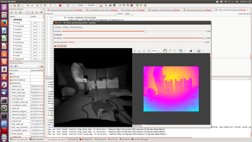
Ubuntu screenshot of the depth image denoising application
The demonstration video first shows the different parts of this video processing algorithm: first the non-local means denoising algorithm used for processing depth images, second the rendering functionality (through OpenGL vertex buffers) and finally, the user interface code (with sliders, labels and displays).
When the program runs, first a flat 2D image is shown on the left, together with the depth image on the right. By adjusting the “3D” slider, the flat image is extruded to a 3D surface.
It can be seen that there are some problems in the resulting 3D mesh, especially in the vicinity of right hand of the test subject. These problems are caused by reflective properties of the desk lamp standing in between the subject and the camera. By increasing the denoising level of the algorithm, this problem can easily be solved. Although the 3D surface has a much smoother appeareance, the depth image on the right reveals that the depth image is actually over-smoothed. The right balance between smoothing and local surface artifacts can be found by setting the denoising level somewhere “in the middle”.